Introduction:
This article is the first part of a series on time series prediction for cryptocurrency financial data. This article focuses on evaluating different preprocessing techniques for Bitcoin pricing data.
By labeling Bitcoin price sequences into three classes – buy, sell, and hold, I intend to create models capable of predicting short-term price movements using LSTM RNNs. After exploring preprocessing techniques in this article, subsequent articles will dive deeper into network architectures, advanced data techniques, and more.
Preprocessing plays a pivotal role in shaping the structure and characteristics of the data, ultimately affecting the performance of prediction models. The choice of preprocessing can, therefore, substantially influence the resulting predictions.
While the primary goal of this project is to learn more about deep learning, data science, and financial markets, a secondary aim is to derive a model and trading strategy that capitalizes on the available data. The hope is to deploy a successful model in a live environment.
The complete code for this project is accessible on my GitHub.
Preliminaries:
Data:
The data used for this project are Bitcoin’s 5-minute candles spanning June 2016 to June 2023. The short 5-minute candles choice is driven by two factors:
- Expanding the volume of training data for RNNs.
- The hypothesis that short-term market movements, devoid of external influence, might be easier to predict using pricing data only
The dataset comprises of attributes such as low, high, open, close, weightedAverage, and volume. Although post-2021 data offers tradeCount and more, these won’t be used due to their unavailability for the majority of the timeframe. hl_percent refers to the percentage change between high and low.
All data has been sourced from the Poloniex Exchange API, which also offers capabilities to integrate a live trading bot.
| close | hl_percent | weightedAverage | quantity_baseUnits | dt_closeTime |
| 681.84 | 0.005617 | 679.87 | 0.488352 | 2016-07-01 14:10:00 |
| 683.4 | 0.007914 | 682.69 | 0.239165 | 2016-07-01 14:15:00 |
| … | … | … | … | … |
| 30426.45 | 0.0005264 | 30419.85 | 0.205135 | 2023-07-01 08:00:00 |
| 30439.96 | 0.0007049 | 30427.6 | 0.094435 | 2023-07-01 08:05:00 |
Fig. 1: Data used in this article
Labeling Technique:
The ground truth labeling should ideally be done in a way that maximizes returns and minimizes risk while maintaining a set trading frequency. For the purpose of first comparing data preprocessing steps and model architectures, I will stick to something rather simple but sufficient.
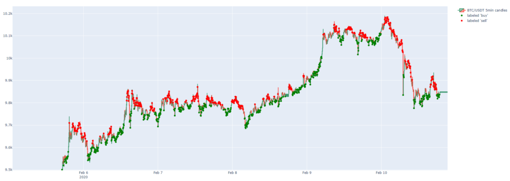
Data points are labeled as buy if two conditions are fulfilled. 1) the average close price of the next 40 candles is higher than the current price by certain threshold. 2) the average close price of the surrounding 80 candles (previous 40 and next 40) is higher than the current price by certain threshold. The second condition ensures that in a rising market not every point is labeled as buy, but only those in valleys at the beggining of the upward movement. Data points are labeled as sell if the surrounding averages are lower, and as hold if the thresholds are not passed.
The threshhold is chosen in a way that balances the amount of labeled buys, sells, and holds to an even distribution of 33% each. This is done in order to maximize the amount of training data. Otherwise, the number of examples in each category would be limited by the category containing the least examples, as the number of training examples need to be balanced.
The derived threshold was a 0.04% fluctuation in price in the aforementioned 1.5h timeframe. This number is only the necessary minimum, but is still really small. It would be reasonable to increase it in the future by increasing the look-ahead and making larger market-movement predictions.

Fig. 2: Example of ground truth labeling of training data
After labeling, the data is segmented into sequences lasting 15h each (180 candles). These sequences are then processed by LSTM RNNs to predict their corresponding labels.
Network Architecture:
The network architecture and more will be subject to change in the following articles of this series.

Fig. 3: Basic network architecture
Preprocessing Approaches and Results:
Three preprocessing approaches will be explored. The first two compare wether it works better to preprocess the entire data before subdividing it into seqences, or preprocessing every individual sequence after subdividing. For these approaches, only the features close, hl_percent and quantity_baseUnits will be used.
The third approach builds on the better one of the previous two (the first one). Additionally, it introduces more features and a log transform.
1. Global Preprocessing (prior to sequencing):
This is the fundamental approach where preprocessing is applied uniformly across the entire dataset before breaking it down into sequences. One main advantage of this method is the uniformity of preprocessing, ensuring that relative changes between sequences stay intact.
It’s crucial to scale the training data first and afterwards apply the same scaling parameters to the validation data to prevent data leakage.
Techniques used:
- Percentage Change: By computing the percentage change, we transition the original price features into a format that represents relative changes from candle to candle, aiding in making the data more stationary.
- Scaling: Normalizing the data ensures that values have a 0 mean and a unit variance, a form suitable for most algorithms, especially neural networks.
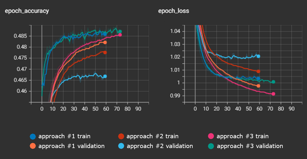
A train- and validation accuracy of >48% was achieved. The results are shown in Figure 4.
2. Local Preprocessing (post sequencing):
In contrast to the global approach, here, preprocessing is applied individually to each sequence after the dataset is broken down. One potential benefit is the increased robustness against variations in the individual sequences. Everything else is kept the same. A percent change transform is applied and afterwards each sequence is scaled to 0 mean and unit variance.
The results of this method are slightly worse than those of the first (see Fig. 4). This indicates that the inter-sequence differences, that are better maintained by global preprocessing, are more beneficial for the model than the more standardized sequences of this second approach. Finding a balance between these two approaches may be further explored in the future by utilizing change point detection; larger chunks of the data – corresponding to different market dynamics (e.g. bear-/bull market or low/high volatility) – may be preprocessed individually.
3. Global Preprocessing with additional Features:
Building on the strengths of global preprocessing, this method introduces additional features and a log transform before the percentage change. Applying the log transform can help stabilize the variance across the dataset. This can benefit time series data, especially when dealing with multiplicative seasonality or exponential trends. It can also make outlier effects less pronounced.
As before, it remains crucial to scale only the training data first and apply the same scaling parameters to the validation data to prevent data leakage.
Including the other pricing features open, low, and high did not have an effect on the performance of the model. This was in part expected, as the open feature is the same as the close feature, just shifted forward by one row. Additionally, including low and high having no impact on the performance, supports the assumption that their relevant information is already included in the hl_percent feature.
Including the weightedAverage for each candle did however increase the model’s performance. This makes sense, as it introduces new information about the price development during the 5min candle interval.

Fig. 4: Train- and validation results